instructor :

​ Loannis Gkioulekas . Yannis

# lecture 1

# Linear shift-invariant image filtering

线性性（Linearity）: 线性系统满足叠加原理，即对于输入信号 $f_1$ 和 $f_2$ 以及常数 $a$ 和 $b$，有：

$$L(af_1 + bf_2) = aL(f_1) + bL(f_2)$$

其中，$L$ 表示线性系统。

平移不变性（Shift-Invariance）: 平移不变性表示系统的特性不随输入信号的位置改变而改变。即如果输入信号 $f(x,y)$ 平移了 $(x_0, y_0)$，则输出信号也相应平移相同的量：

$$L(f(x - x_0, y - y_0)) = L(f)(x - x_0, y - y_0)$$

在图像处理中，线性平移不变滤波通常用卷积操作来表示:

# 均值滤波器（Mean Filtering）

主要用于平滑图像，减少噪声。其基本思想是用一个卷积核（通常是一个大小为 n×nn \times nn×n 的矩阵）在图像上移动，每个像素点的值用其邻域内所有像素的平均值代替。

##### 操作步骤：

1. 确定卷积核的大小（如 3x3, 5x5）。
2. 对图像中的每个像素点，计算其邻域内所有像素的平均值。
3. 用计算得到的平均值代替当前像素点的值。

$$(I * h)(x, y) = \frac{1}{N} \sum_{i=-\frac{N}{2}}^{\frac{N}{2}} \sum_{j=-\frac{N}{2}}^{\frac{N}{2}} I(x-i, y-j)$$

# 高斯滤波器（Gaussian Filtering）

基于高斯函数的线性滤波器，主要用于图像平滑和模糊处理。其特点是能保留图像的边缘细节，较少产生伪影。

# 操作步骤：

1. 确定高斯核的大小和标准差（σ）。
2. 生成高斯核，根据高斯函数计算每个核值。
3. 使用高斯核对图像进行卷积操作，计算邻域内像素的加权平均值。

$$(I * h)(x, y) = \frac{1}{N} \sum_{i=-\frac{N}{2}}^{\frac{N}{2}} \sum_{j=-\frac{N}{2}}^{\frac{N}{2}} I(x-i, y-j)$$

# 中值滤波器（Median Filtering）

非线性滤波器，主要用于去除图像中的椒盐噪声。它通过取邻域内所有像素值的中值来替代当前像素点的值。

$$(I * h)(x, y) = \text{median}\{ I(x+i, y+j) \mid -\frac{N}{2} \leq i, j \leq \frac{N}{2} \}$$

# 操作步骤：

1. 确定滤波窗口的大小（如 3x3, 5x5）。
2. 对图像中的每个像素点，取其邻域内所有像素值。
3. 计算这些值的中值，用该中值替代当前像素点的值。

# Sobel 滤波器（Sobel Filter）

边缘检测滤波器，主要用于检测图像中的边缘。它通过计算梯度的大小和方向来识别图像中的显著变化。

# 操作步骤：

1. 使用两个 3x3 的 Sobel 核，分别检测水平和垂直方向上的梯度。
2. 对图像进行卷积操作，分别计算水平和垂直方向上的梯度图像。
3. 计算梯度的大小和方向，得到边缘图像。

水平梯度：

$$G_x = \begin{bmatrix} -1 & 0 & 1 \\ -2 & 0 & 2 \\ -1 & 0 & 1 \end{bmatrix} * I$$

垂直梯度：

$$G_y = \begin{bmatrix} -1 & -2 & -1 \\ 0 & 0 & 0 \\ 1 & 2 & 1 \end{bmatrix} * I$$

综合梯度：

$$G = \sqrt{G_x^2 + G_y^2}$$

# 拉普拉斯滤波器（Laplacian Filter）

边缘检测滤波器，它通过计算图像的二阶导数来检测边缘。该滤波器对噪声敏感，通常在使用前需要对图像进行平滑处理.

# 操作步骤：

1. 使用一个拉普拉斯核（如 3x3 的矩阵）。

2. 对图像进行卷积操作，计算每个像素点的拉普拉斯值。

3. 对拉普拉斯值进行阈值处理，得到二值化的边缘图像。

   $$h(i, j) = \begin{bmatrix} 0 & 1 & 0 \\ 1 & -4 & 1 \\ 0 & 1 & 0 \end{bmatrix} * I$$

# 方框滤波器 （Box Filter)

是一种特殊的均值滤波器，其中每个卷积核元素的值相等，且其和为 1。与均值滤波器类似

Box Filter 与均值滤波器的公式相同：

$$(I * h)(x, y) = \frac{1}{N} \sum_{i=-\frac{N}{2}}^{\frac{N}{2}} \sum_{j=-\frac{N}{2}}^{\frac{N}{2}} I(x-i, y-j)$$

####box filter

# 2D planar and linear transformations

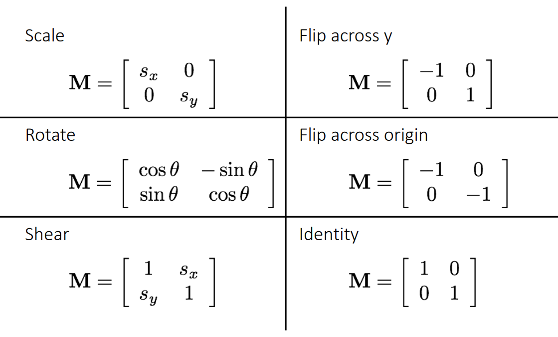
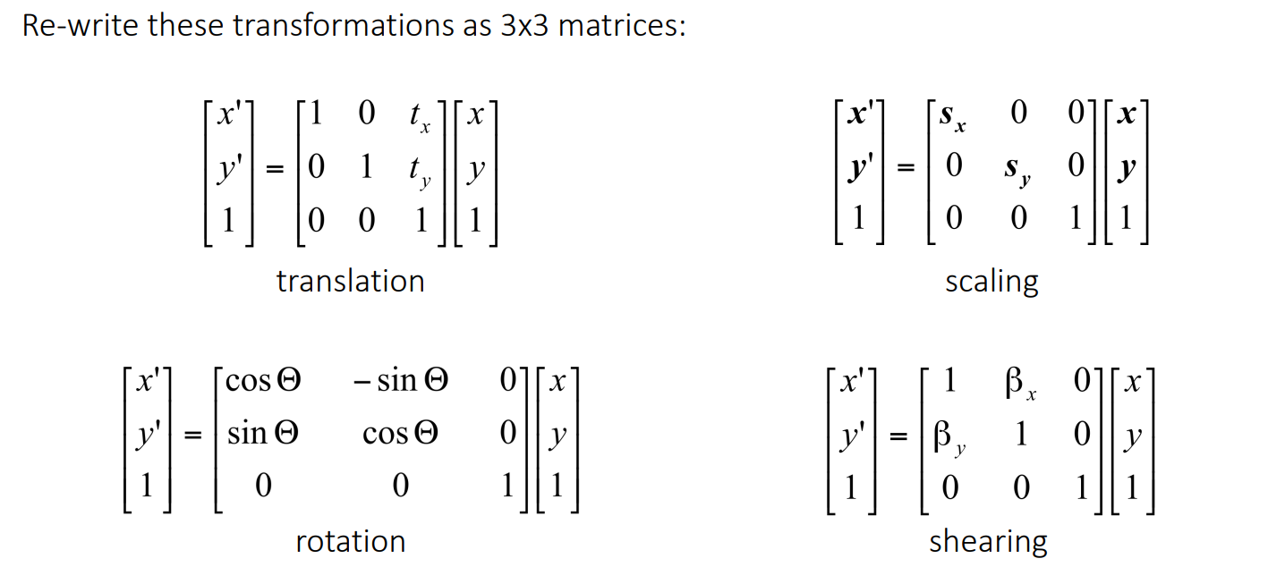
# Homogeneous coordinates

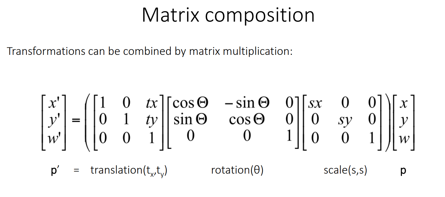
Multiplication order matters! Transformations are applied from right to left.

# Classification of 2D transformations

# Translation 2

\ \begin{pmatrix} x' \\ y' \end{pmatrix} = \begin{pmatrix} 1 & 0 & t_x \\ 0 & 1 & t_y \\ 0 & 0 & 1 \end{pmatrix} \begin{pmatrix} x \\ y \\ 1 \end{pmatrix} \

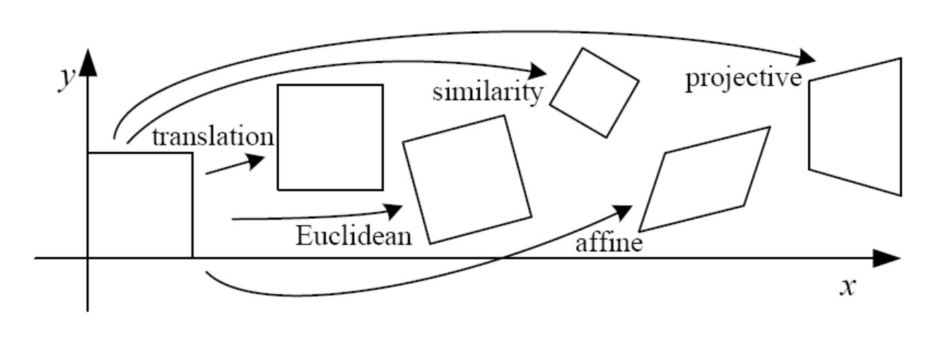
# Euclidean 3

$$\begin{pmatrix} x' \\ y' \end{pmatrix} = \begin{pmatrix} \cos \theta & -\sin \theta & t_x \\ \sin \theta & \cos \theta & t_y \\ 0 & 0 & 1 \end{pmatrix} \begin{pmatrix} x \\ y \\ 1 \end{pmatrix}$$

# Similarity 4

$$\begin{pmatrix} x' \\ y' \end{pmatrix} = \begin{pmatrix} s \cos \theta & -s \sin \theta & t_x \\ s \sin \theta & s \cos \theta & t_y \\ 0 & 0 & 1 \end{pmatrix} \begin{pmatrix} x \\ y \\ 1 \end{pmatrix}$$

# Affine 6

$$\begin{pmatrix} x' \\ y' \end{pmatrix} = \begin{pmatrix} a & b & t_x \\ c & d & t_y \\ 0 & 0 & 1 \end{pmatrix} \begin{pmatrix} x \\ y \\ 1 \end{pmatrix}$$

# Projective 8

$$\begin{pmatrix} x' \\ y' \\ w \end{pmatrix} = \begin{pmatrix} a & b & c \\ d & e & f \\ g & h & 1 \end{pmatrix} \begin{pmatrix} x \\ y \\ 1 \end{pmatrix}$$

# Solving linear systems

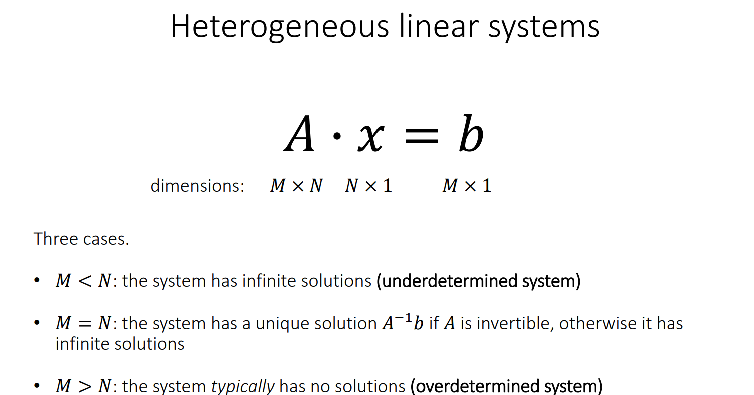
# Heterogeneous linear systems

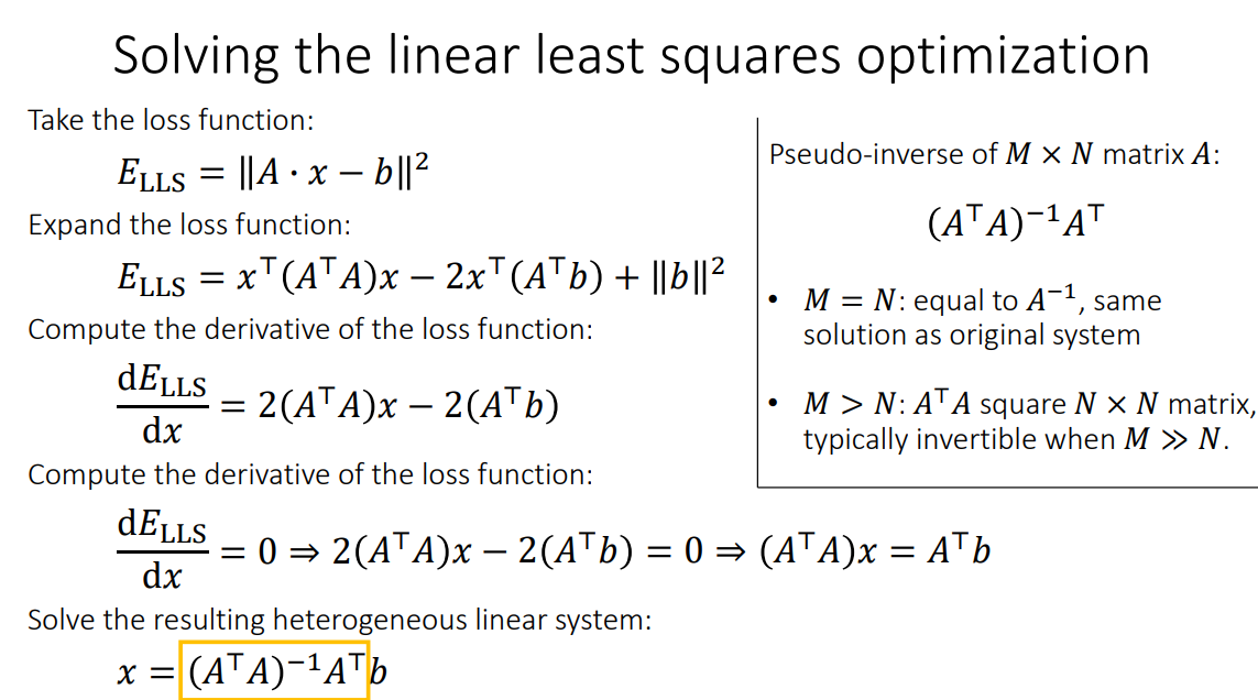
with the optimization problem:

$$\min_{\mathbf{x}} \| A \mathbf{x} - \mathbf{b} \|^2$$

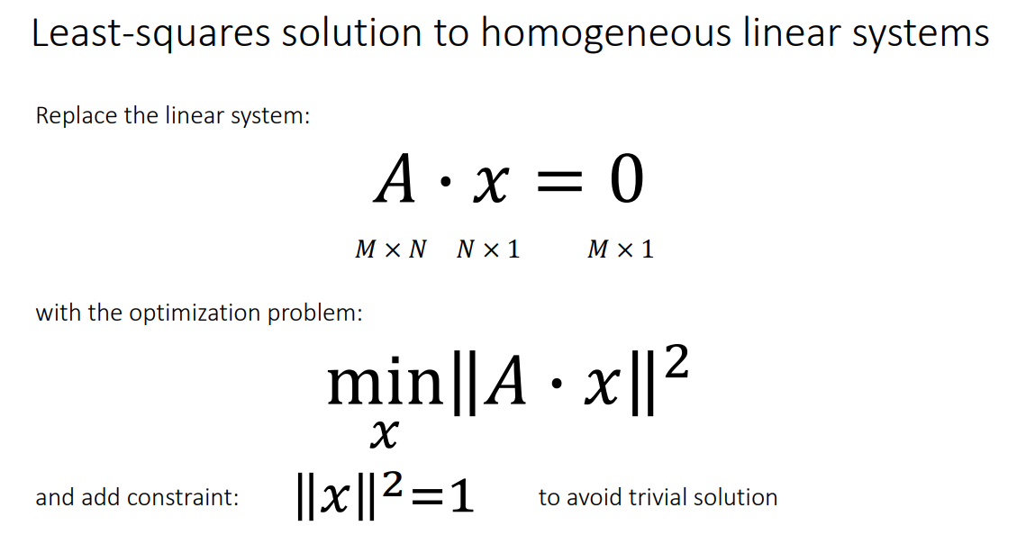
# Homogeneous linear systems

# 解决问题

• image A and B, find a way of transform to aligns image B to image A.
• Support we have already find 4 pairs of corresponding points by some method:
  A:$ (x_1, y_1), (x_2, y_2), (x_3, y_3), (x_4, y_4)$

​ B:$(x_1', y_1'), (x_2', y_2'), (x_3', y_3'), (x_4', y_4')$

We wish to find an affine transformation matrix T :

$$\begin{pmatrix} x' \\ y' \\ 1 \end{pmatrix} = \begin{pmatrix} a & b & c \\ d & e & f \\ 0 & 0 & 1 \end{pmatrix} \begin{pmatrix} x \\ y \\ 1 \end{pmatrix}$$

We can expand the matrix equation into two linear equations:

$$\begin{cases} x' = ax + by + c \\ y' = dx + ey + f \end{cases}$$

For each pair of corresponding points, we have a set of such equations. For four pairs of corresponding points, we have eight equations:

$$\begin{cases} x_1' = ax_1 + by_1 + c \\ y_1' = dx_1 + ey_1 + f \\ x_2' = ax_2 + by_2 + c \\ y_2' = dx_2 + ey_2 + f \\ x_3' = ax_3 + by_3 + c \\ y_3' = dx_3 + ey_3 + f \\ x_4' = ax_4 + by_4 + c \\ y_4' = dx_4 + dy_4 + f \end{cases}$$

We can write these equations in matrix form $A \mathbf{x} = \mathbf{b}$, where:

$$A = \begin{pmatrix} x_1 & y_1 & 1 & 0 & 0 & 0 \\ 0 & 0 & 0 & x_1 & y_1 & 1 \\ x_2 & y_2 & 1 & 0 & 0 & 0 \\ 0 & 0 & 0 & x_2 & y_2 & 1 \\ x_3 & y_3 & 1 & 0 & 0 & 0 \\ 0 & 0 & 0 & x_3 & y_3 & 1 \\ x_4 & y_4 & 1 & 0 & 0 & 0 \\ 0 & 0 & 0 & x_4 & y_4 & 1 \\ \end{pmatrix}$$

$$\mathbf{x} = \begin{pmatrix} a \\ b \\ c \\ d \\ e \\ f \end{pmatrix}$$

$$\mathbf{b} = \begin{pmatrix} x_1' \\ y_1' \\ x_2' \\ y_2' \\ x_3' \\ y_3' \\ x_4' \\ y_4' \end{pmatrix}$$

通过求解正常方程 $A^TAx=ATb $，我们可以得到最小二乘解 X.

# Eigenvector

$$Av=λv$$

对于一个矩阵 A，如果存在一个非零向量 $v$ 和一个标量 $λ$ 使得$Av=λv$，那么 $v$ 就是 A 的特征向量，$λ$ 是对应的特征值。

# SVD

$$A=UΣV^T$$

$U$: Left Singular Vectors for $AA^T$ $U=[u1,u2,…,uM]$

$Σ$: Singular Values

$$\Sigma = \begin{pmatrix} \sigma_1 & 0 & \cdots & 0 \\ 0 & \sigma_2 & \cdots & 0 \\ \vdots & \vdots & \ddots & \vdots \\ 0 & 0 & \cdots & \sigma_r \end{pmatrix} \quad where\quad \sigma_i = \sqrt{\lambda_i}$$

$V$: Right Singular Vectors for $A^TA$ $V=[v1,v2,…,vN]$

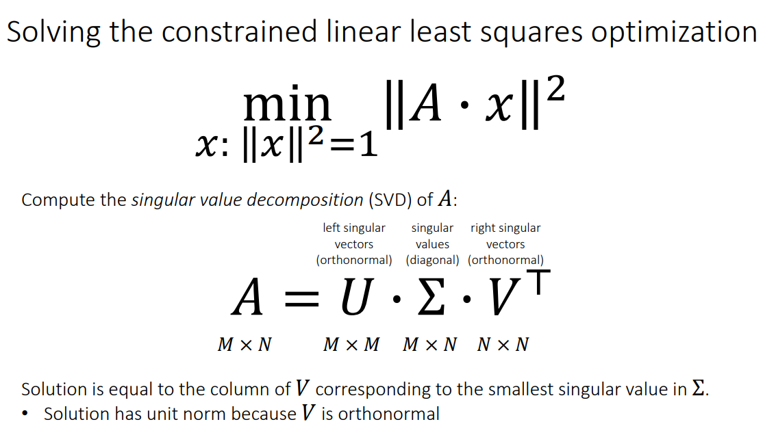
为了最小化 $∥Ax∥^2$ 并满足 $∥x∥^2=1$，我们可以利用 SVD 的结果：

1. 将优化问题转换为标准形式： 通过 SVD，我们可以将原优化问题转化为：

   $$∥Ax∥^2=∥UΣVTx∥^2$$

   因为 $U$ 是正交矩阵，保持向量的范数不变，所以我们可以忽略 $U$：

   $$\min⁡_{\mathbf{x}}∥ΣV^Tx∥^2$$

2. 定义新变量： 令 $ y=V^Tx$，则 $y$ 也是一个单位向量（因为 $V$ 是正交矩阵）。我们需要最小化：

   $$∥Σy∥^2$$

3. 选择最小奇异值对应的方向： $Σ$ 是一个对角矩阵，其中的奇异值按降序排列。为了使 $∥Σy∥^2$ 最小，$y$ 应该选择与最小奇异值对应的方向。

4. 恢复原变量： 最后，利用 $y=V^Tx$，我们可以求出满足 $∥x∥^2=1$ 的 $x$

###Basic reading

• Szeliski textbook, Sections 2.1, 3.6.
• Hartley and Zisserman textbook, Section 2.

# lecture 2